Quick start
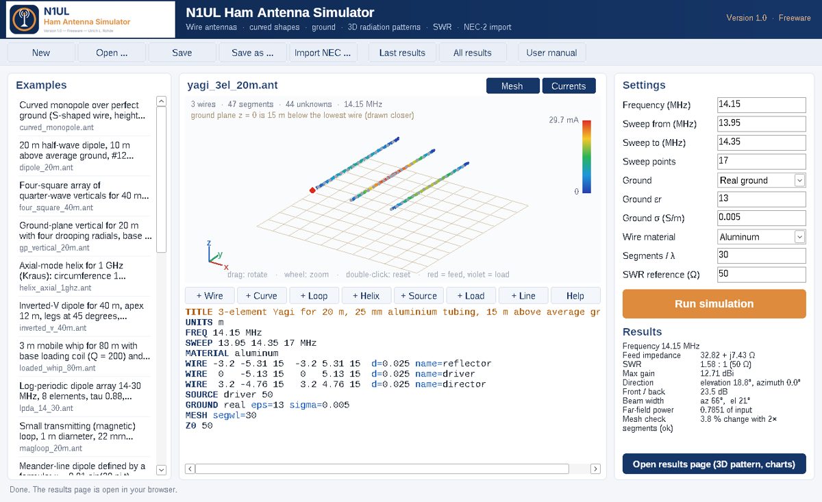
- Open an example (Examples list on the left) or write a model in the editor, one command per line;
#starts a comment. - The 3D view shows the wires as you type (feed points red, loads violet). Drag to rotate, wheel to zoom, double-click to reset.
- The buttons + Wire, + Curve, + Loop, + Helix, + Source, + Load, + Line insert a template line that you then edit.
- Press Run simulation. The results open in your web browser; the button ◀ Back to the program at the top of the results page brings this window back.
- Save the model with Save; models are plain text files (.ant). NEC-2 card decks (.nec) are read directly.
Commands
Lengths are in the unit set by UNITS (default metre). Square brackets mark optional parts; | separates alternatives.
| Command | Syntax | What it does | Example |
|---|---|---|---|
| TITLE | TITLE text | Name of the model (shown on the results page). | TITLE 3-element Yagi for 20 m |
| UNITS | UNITS m | cm | mm | ft | in | Length unit for all following numbers (default m). | UNITS mm |
| FREQ | FREQ f MHz | Design frequency: radiation pattern, currents, matching network. | FREQ 14.15 MHz |
| SWEEP | SWEEP f1 f2 n MHz | Frequency sweep with n points: impedance, SWR / return loss, gain. | SWEEP 13.9 14.4 26 MHz |
| WIRE | WIRE x1 y1 z1 x2 y2 z2 d=.. | r=.. | awg=.. [seg=n] [name=..] [mat=..] | Straight wire from point 1 to point 2; size by diameter d, radius r or AWG gauge. | WIRE 0 -5.13 15 0 5.13 15 d=0.02 name=driven |
| SPLINE | SPLINE x1 y1 z1 x2 y2 z2 ... d=.. name=.. | Smooth curved wire through the given points. | SPLINE 0 0 0 0.5 0 1 0 0 2 d=0.004 |
| POLYLINE | POLYLINE x1 y1 z1 ... d=.. name=.. | Straight pieces through the given points (bent wires, zig-zags). | POLYLINE 0 0 0 1 0 0 1 1 0 d=0.002 |
| CURVE | CURVE "x(t)" "y(t)" "z(t)" [t0=0 t1=1] d=.. name=.. | Wire along a formula (sin, cos, exp, sqrt, pi ...). | CURVE "0.5*cos(2*pi*t)" "0.5*sin(2*pi*t)" "0.1*t" d=0.003 |
| LOOP | LOOP cx cy cz radius sides [axis=x|y|z] [rot=deg] d=.. name=.. | Closed loop (polygon with many sides) around a centre. | LOOP 0 0 1.5 0.5 24 axis=y d=0.022 name=loop |
| HELIX | HELIX x y z radius pitch turns [sides=16] [left] d=.. name=.. | Helix along z; "left" for left-hand winding. | HELIX 0 0 0 0.05 0.075 8 d=0.002 |
| DISH | DISH D=.. F=.. | FD=.. [mesh=..] [wire=..] [block=..] | Parabolic reflector (physical optics), focus at the origin, opening toward +z; the feed wires are modelled normally. Optional wire mesh and central blockage. | DISH D=43 FD=0.4 mesh=5cm wire=2mm block=1 |
| SOURCE | SOURCE wire pos% [V=1] [phase=deg] | Voltage source on a wire (name or number), position 0 ... 100 % from the first end. | SOURCE driven 50 |
| LOAD | LOAD wire pos% R=.. L=.. C=.. [par] or X=.. | Lumped load (series R-L-C, or parallel with "par"), or a fixed reactance X. | LOAD mast 100 L=60.8e-6 R=7.2 |
| TL | TL wire1 pos1% wire2 pos2% Z0=.. [len=..] [vf=..] [loss=dB/100m] [rev] | Transmission line between two points (phasing lines, stubs). | TL e1 50 e2 50 Z0=75 len=3.5 vf=0.66 |
| GROUND | GROUND free | perfect | real eps=.. sigma=.. [sommerfeld] | Ground below z = 0. "sommerfeld": exact near field of the ground (antennas lower than about 0.1 wavelength). | GROUND real eps=13 sigma=0.005 sommerfeld |
| GROUND pcb | GROUND pcb eps=4.4 tand=0.02 h=1.6mm [groundplane] | Printed board, top surface at z = 0 (strips are drawn as wires in the plane). | GROUND pcb eps=4.4 tand=0.02 h=1.6mm groundplane |
| MATERIAL | MATERIAL perfect | copper | aluminum | brass | steel | stainless | silver | Conductor of all following wires (or per wire with mat=..). | MATERIAL copper |
| MESH | MESH segwl=30 [taper=on|off] | Segments per wavelength; tapering refines the mesh at feeds and junctions. | MESH segwl=40 |
| Z0 | Z0 50 | Reference impedance for SWR and return loss. | Z0 50 |
| PATTERN | PATTERN dth=2 dph=5 | Angular grid of the radiation pattern (degrees). | PATTERN dth=1 dph=2 |
| VAR | VAR name=value ... | Named variables, usable in any number. | VAR L=5.13 h=15 |
| OPTVAR | OPTVAR name min max | Variable that "Run" optimizes between the limits. | OPTVAR L 4.9 5.4 |
| GOAL | GOAL gmax | gain elev=.. az=.. | fb target=.. | swr target=.. | r target=.. | x [weight=1] | Optimization goal(s). | GOAL swr target=1.5 weight=2 |
| OPTSET | OPTSET pop=30 gen=40 seed=1 | Optimizer settings (differential evolution). | OPTSET pop=40 gen=60 |
NEC-2 card decks (.nec: GW GA GH GM GR GX GS GE GN EX LD TL NT FR) are read directly.
Examples with pictures
Each example is in the Examples folder; the picture shows part of its results page.
3-element Yagi for 20 m
TITLE 3-element Yagi for 20 m, 25 mm aluminium tubing, 15 m above average ground
UNITS m
FREQ 14.15 MHz
SWEEP 13.95 14.35 17 MHz
MATERIAL aluminum
WIRE -3.2 -5.31 15  -3.2 5.31 15  d=0.025 name=reflector
WIRE  0   -5.13 15   0   5.13 15  d=0.025 name=driver
WIRE  3.2 -4.76 15   3.2 4.76 15  d=0.025 name=director
SOURCE driver 50
GROUND real eps=13 sigma=0.005
Examples\yagi_3el_20m.ant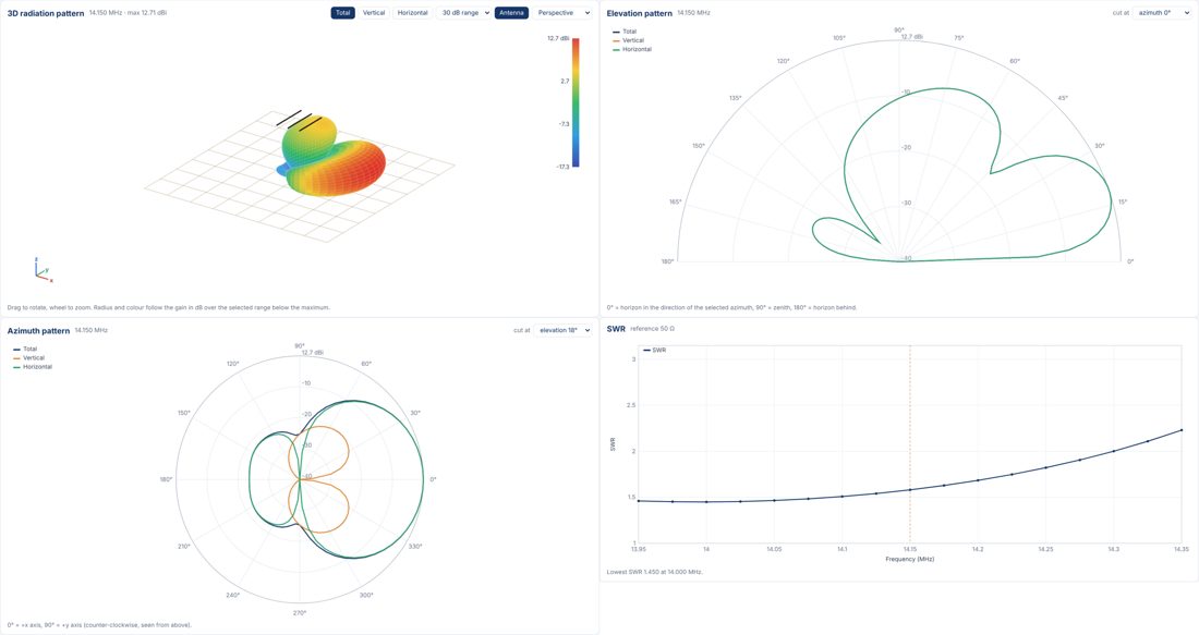
Half-wave dipole for 20 m
TITLE 20 m half-wave dipole, 10 m above average ground, #12 copper wire
UNITS m
FREQ 14.175 MHz
SWEEP 13.9 14.45 23 MHz
WIRE -5.13 0 10  5.13 0 10  awg=12 name=dipole
SOURCE dipole 50
GROUND real eps=13 sigma=0.005
MATERIAL copper
Examples\dipole_20m.ant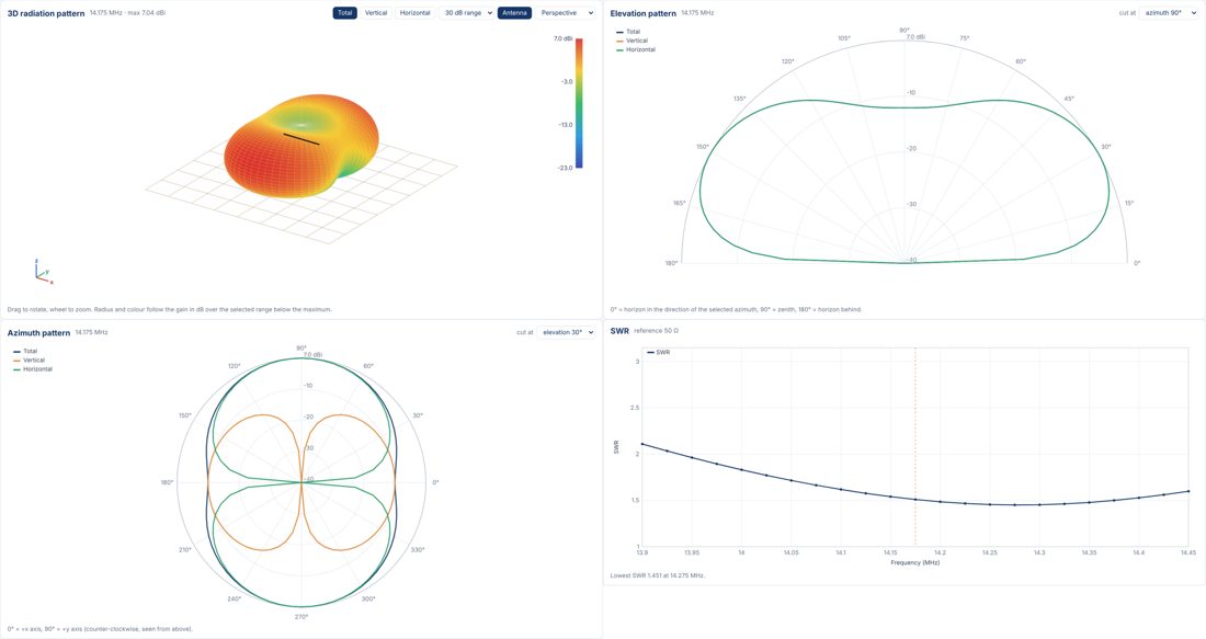
Small magnetic loop for 20 m
TITLE Small transmitting (magnetic) loop, 1 m diameter, 22 mm copper tube, tuned to 14.1 MHz by a 47.7 pF capacitor (series feed, R = 0.14 ohm)
UNITS m
FREQ 14.1 MHz
SWEEP 13.9 14.3 41 MHz
MATERIAL copper
LOOP 0 0 3  0.5 24 axis=x d=0.022 name=lp rot=-90
SOURCE lp1 0
LOAD lp13 0 C=47.7e-12
GROUND real eps=13 sigma=0.005
Examples\magloop_20m.ant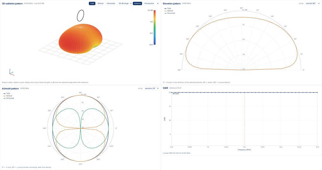
3 m mobile whip for 80 m with loading coil
TITLE 3 m mobile whip for 80 m with base loading coil (Q = 200) and 10 ohm ground loss, perfect ground
UNITS m
FREQ 3.75 MHz
SWEEP 3.7 3.8 21 MHz
MATERIAL steel
WIRE 0 0 0  0 0 0.3  d=0.025 name=mast
WIRE 0 0 0.3  0 0 3.3  d=0.008 name=whip
SOURCE mast 0
LOAD mast 100 L=60.8e-6 R=7.2
LOAD mast 0 R=10
GROUND perfect
Examples\loaded_whip_80m.ant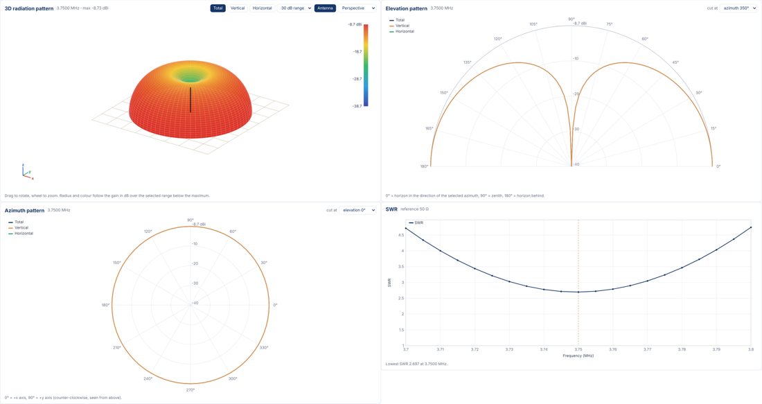
Axial-mode helix, circular polarisation, 1 GHz
TITLE Axial-mode helix for 1 GHz (Kraus): circumference 1 wavelength, 13 deg pitch, 6 turns, over a ground plane
UNITS m
FREQ 1.0 GHz
SWEEP 0.8 1.2 21 GHz
WIRE 0.0477 0 0  0.0477 0 0.01  r=0.001 name=feed
HELIX 0 0 0.01  0.0477 0.0697 6  sides=20 r=0.001 name=h
SOURCE feed 0
GROUND perfect
Examples\helix_axial_1ghz.ant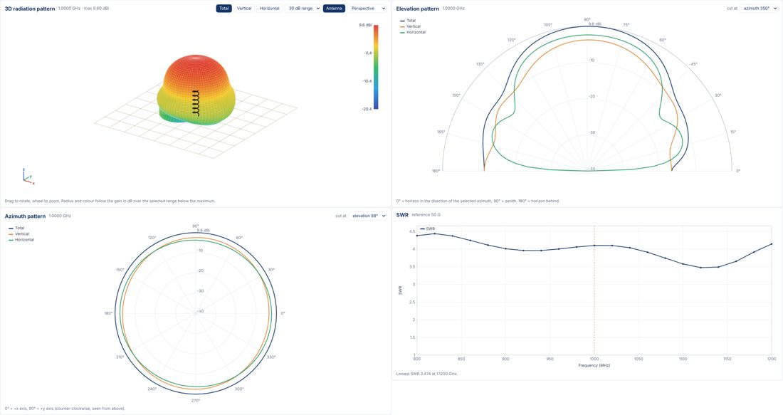
Log-periodic dipole array 14-30 MHz
TITLE Log-periodic dipole array 14-30 MHz, 8 elements, tau 0.88, sigma 0.06, 100 ohm crossed feeder
UNITS m
FREQ 21.2 MHz
SWEEP 14 30 33 MHz
MATERIAL aluminum
WIRE 0.000 -5.700 15  0.000 5.700 15  d=0.02 name=e1
WIRE 1.368 -5.016 15  1.368 5.016 15  d=0.02 name=e2
WIRE 2.572 -4.414 15  2.572 4.414 15  d=0.02 name=e3
WIRE 3.631 -3.884 15  3.631 3.884 15  d=0.02 name=e4
WIRE 4.564 -3.418 15  4.564 3.418 15  d=0.02 name=e5
WIRE 5.384 -3.008 15  5.384 3.008 15  d=0.02 name=e6
WIRE 6.106 -2.647 15  6.106 2.647 15  d=0.02 name=e7
WIRE 6.741 -2.329 15  6.741 2.329 15  d=0.02 name=e8
TL e1 50 e2 50 Z0=100 rev
TL e2 50 e3 50 Z0=100 rev
TL e3 50 e4 50 Z0=100 rev
TL e4 50 e5 50 Z0=100 rev
TL e5 50 e6 50 Z0=100 rev
TL e6 50 e7 50 Z0=100 rev
TL e7 50 e8 50 Z0=100 rev
SOURCE e8 50
Z0 100
GROUND real eps=13 sigma=0.005
Examples\lpda_14_30.ant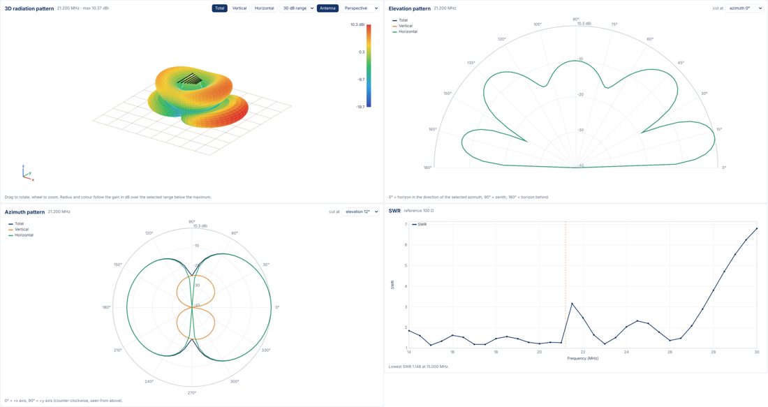
Parabolic dish, 43 m at 435 MHz
TITLE 43 m parabolic dish at 435 MHz, prime-focus dipole feed with a reflector screen (sketch)
UNITS m
FREQ 435 MHz
SWEEP 425 445 5 MHz
MATERIAL aluminum
# feed at the focus (origin): half-wave dipole along x, illuminating the dish below it (-z)
WIRE -0.164 0 0      0.164 0 0      dmm=12 name=dipole
SOURCE dipole 50
# reflector screen 0.15 m behind the dipole: five rods, 0.5 m long, 0.15 m apart
WIRE -0.25 -0.30 0.15  0.25 -0.30 0.15  dmm=10
WIRE -0.25 -0.15 0.15  0.25 -0.15 0.15  dmm=10
WIRE -0.25  0.00 0.15  0.25  0.00 0.15  dmm=10
WIRE -0.25  0.15 0.15  0.25  0.15 0.15  dmm=10
WIRE -0.25  0.30 0.15  0.25  0.30 0.15  dmm=10
# reflector: 43 m diameter, F/D = 0.4 (focal length 17.2 m, vertex 17.2 m below the feed),
# wire mesh with 5 cm cells of 2 mm wire, 1 m central blockage by the feed housing.
# The focal length and the mesh are assumptions: put in the values of the real dish.
DISH D=43 FD=0.4 mesh=5cm wire=2mm block=1
PATTERN dth=2 dph=5
Examples\dish_43m_435MHz.antThe dipole and its reflector screen are the feed at the focus; DISH adds the reflector. The results page then has the view Parabolic reflector with gain, aperture, spillover and illumination efficiency, edge illumination, beam widths and side lobes, and the 3D pattern with the dish drawn to scale.
Magnetic loops (small transmitting loops)
A magnetic loop is a LOOP of thick tube tuned by a capacitor (LOAD ... C= R=, with R = XC/QC for the capacitor loss) and fed by a small Faraday coupling loop, which is simply a second, smaller LOOP carrying the SOURCE. Examples: magloop_faraday_40m (2 m loop), magloop_faraday_30m and magloop_faraday_20m (1 m loop). Tune the capacitor for resonance (lowest SWR at FREQ) and the coupling-loop diameter for 50 Ω (the input resistance grows with about the fourth power of its diameter). Use a narrow SWEEP (about ±0.2 %), the bandwidth is only a few kHz.
Faraday-fed loop for 20 m
TITLE Small transmitting loop (magnetic loop) for 14.1 MHz: 1 m diameter, 22 mm copper tube, 24-sided, Faraday coupling loop 11.4 cm
# Main loop in the y-z plane, centre 2 m above average ground; tuning capacitor at the top (opposite the feed).
# Faraday coupling loop (11.4 cm, 6 mm conductor) in the same plane at the bottom, 2 cm inside the main loop; the source is in the coupling loop.
# Capacitor 47.50 pF tuned for resonance at 14.1 MHz; its loss is a series resistance Xc/Qc with Qc = 3000 (good air-variable capacitor).
# Coupling-loop size chosen for SWR 1.0 (50 ohm) at 14.1 MHz. Literature: ARRL Antenna Book, small transmitting loops; Balanis, Antenna Theory, ch. 5.
UNITS m
FREQ 14.1 MHz
SWEEP 14.0718 14.1282 201 MHz
MATERIAL copper
LOOP 0 0 2  0.5 24 axis=x d=0.022 name=lp rot=-90
LOOP 0 0 1.57691  0.056913 16 axis=x d=0.006 name=cl rot=-90
SOURCE cl1 0
LOAD lp13 0 C=4.75037e-11 R=0.079205
GROUND real eps=13 sigma=0.005
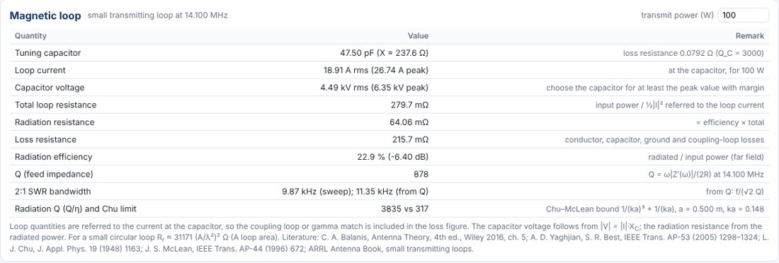
The results page then has the view Magnetic loop: loop current and capacitor voltage at a transmit power you enter, total, radiation and loss resistance, efficiency, Q, 2:1 bandwidth and the Chu–McLean limit.
Near field and RF exposure
The view Near field (for every antenna) shows |E|, |H| or the wave impedance in a plane through the antenna for the power you enter, relative to the FCC or ICNIRP 2020 reference levels, with the distance beyond which both fields are below the limit. Below 30 MHz both E and H must be below the reference level. The near field is computed from the wire currents (exact element fields); far away it equals the radiation pattern.
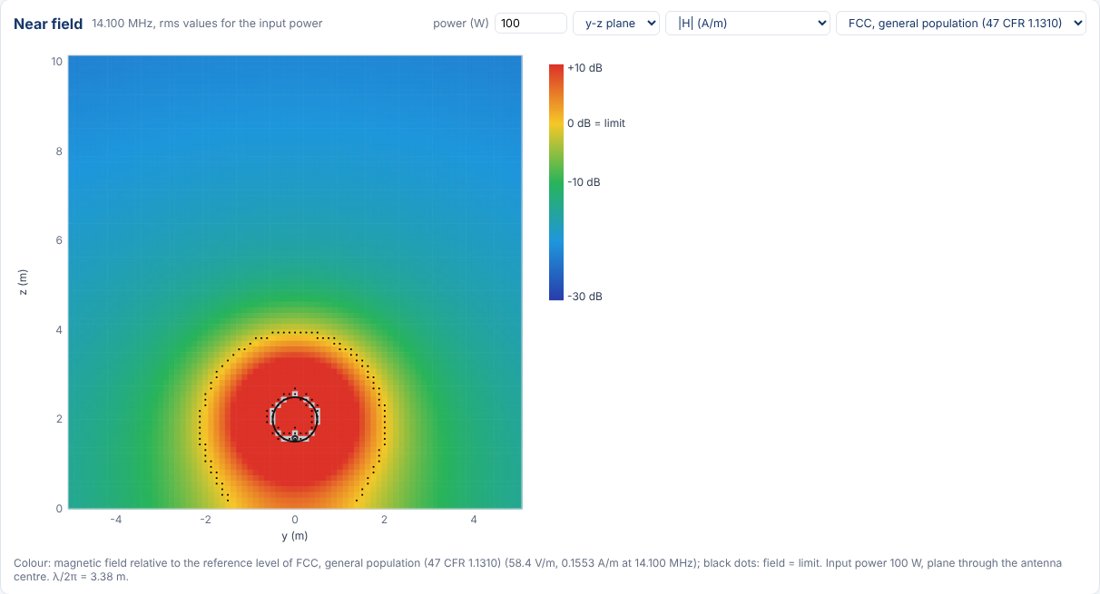
How to use the view is described in the User Manual, Section 9.7; the method and its limits are summarized on the results page itself, under Method and limits. Magnetic loops: User Manual, Section 9.6.
The results page
- Cards at the top: frequency, feed impedance, SWR, gain, direction, front/back, beam width and the matching network.
- SWR: the button pair SWR / Return loss switches the plotted quantity; the other one is shown on the right axis. Hover the chart for values.
- Matching network: the L networks that match the antenna to the line. The low-pass network (series inductor, shunt capacitor) is recommended for transmitting because it attenuates harmonics; the high-pass network (series capacitor, shunt inductor) attenuates lower frequencies (strong broadcast signals, noise) and gives a DC path to ground. A table lists the attenuation of each network at f/2, 2f and 3f when the sweep covers these frequencies.
- Near field: E, H and wave impedance near the antenna, RF exposure distances (FCC, ICNIRP 2020).
- Magnetic loop (when the model has a loop with a tuning capacitor): loop current, capacitor voltage, resistances, efficiency, Q and bandwidth.
- Currents, Smith chart, Feed impedance, Gain vs frequency, Geometry and mesh, the input file and the simulator output.
Tips
- "segment length / radius" warning: the thin-wire method needs segments longer than about twice the wire radius. Use fewer segments (smaller
segwlorseg=n) on thick wires, or model a very thick conductor as several thinner wires. - Above a real ground and lower than about 0.1 wavelength, add
sommerfeldtoGROUND real. - For SWR curves, choose a sweep that covers the band; to see harmonic suppression of the matching networks, sweep from f/2 to 3f.
- The first time you press Back to the program, the browser may ask whether it may open the N1UL program; allow it (optionally "always").